With all of the COVID-19 related stress and my quickly-emerging cabin fever, I was glad to see that this week's Tidy Tuesday was a light-hearted dataset. This week we using the schrute package. As stated in the documentation:

"The schrute package has one and only one purpose: share the complete script transcription for The Office (US) television show. Users are encouraged to use the tidy text data for exploration, learning and fun.“

Rather than try to investigate hard-hitting questions about whether Michael's incompetency predicts output at Dunder Mifflin, I decided to use this opportunity to familiarize myself with tidytext, a package designed for text mining. This vignette is a great introduction.

My post and code were also featured on the TidyX Screencast!

As always, you can find my complete code of my Github.

The data

Let's take a look at the data.

glimpse(schrute)
Observations: 55,130
Variables: 12
$ index            <int> 1, 2, 3, 4, 5, 6, 7, 8, 9, 10, 11, 12, 13, 14, 15, 16, 17, 18, 19, 20, 21, …
$ season           <chr> "01", "01", "01", "01", "01", "01", "01", "01", "01", "01", "01", "01", "01…
$ episode          <chr> "01", "01", "01", "01", "01", "01", "01", "01", "01", "01", "01", "01", "01…
$ episode_name     <chr> "Pilot", "Pilot", "Pilot", "Pilot", "Pilot", "Pilot", "Pilot", "Pilot", "Pi…
$ director         <chr> "Ken Kwapis", "Ken Kwapis", "Ken Kwapis", "Ken Kwapis", "Ken Kwapis", "Ken …
$ writer           <chr> "Ricky Gervais;Stephen Merchant;Greg Daniels", "Ricky Gervais;Stephen Merch…
$ character        <chr> "Michael", "Jim", "Michael", "Jim", "Michael", "Michael", "Michael", "Pam",…
$ text             <chr> "All right Jim. Your quarterlies look very good. How are things at the libr…
$ text_w_direction <chr> "All right Jim. Your quarterlies look very good. How are things at the libr…
$ imdb_rating      <dbl> 7.6, 7.6, 7.6, 7.6, 7.6, 7.6, 7.6, 7.6, 7.6, 7.6, 7.6, 7.6, 7.6, 7.6, 7.6, …
$ total_votes      <int> 3706, 3706, 3706, 3706, 3706, 3706, 3706, 3706, 3706, 3706, 3706, 3706, 370…
$ air_date         <fct> 2005-03-24, 2005-03-24, 2005-03-24, 2005-03-24, 2005-03-24, 2005-03-24, 200…

What we have is every line (text) spoken by every character organized by episode and season.

Prepping the data

First, I used unnest_tokens to split the text variable so that each word is in its own row. This turns streams of dialogue into more manageable “tokens.”

# Tokenize dialogue 
token.schrute = schrute %>%
  tidytext::unnest_tokens(word, text)
dplyr::glimpse(token.schrute) #570,450 observations

After that, I used stop_words to generate a list of stop words. These are words that are not useful for analyses (like “the” and “a”).

stop_words = tidytext::stop_words
tidy.token.schrute = token.schrute %>%
  dplyr::anti_join(stop_words, by = 'word') 

Now that we've removed the stop words, we can visualize the most common words in this dataset.

tidy.token.schrute %>%
  dplyr::count(word, sort = TRUE) %>%
  dplyr::filter(n > 400) %>%
  dplyr::mutate(word = stats::reorder(word, n)) %>%
  ggplot2::ggplot(ggplot2::aes(word, n)) +
  ggplot2::geom_col() +
  ggplot2::xlab(NULL) +
  ggplot2::coord_flip() +
  ggplot2::theme_minimal()

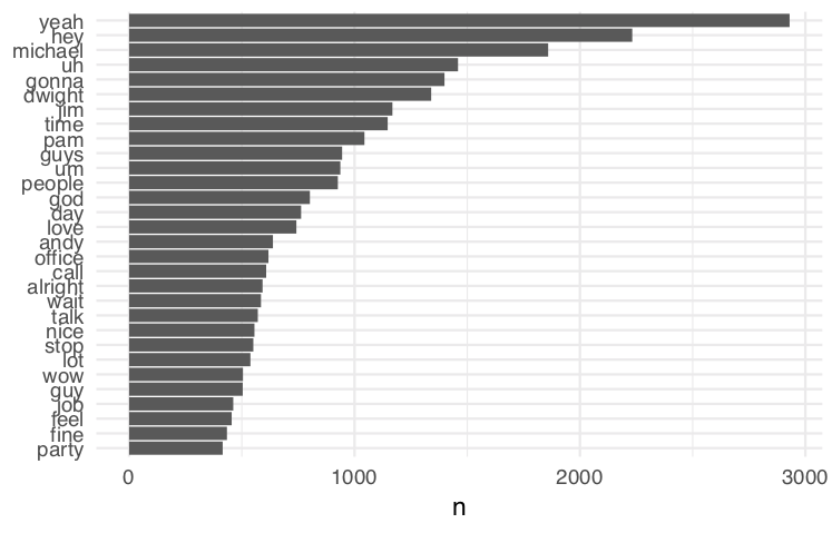
Positive vs Negatively charged words

Now things get interesting! tidytext has a function called get_sentiments that a sentiment lexicon. There are a few you can choose from - I opted for one that determine whether a word has a positive or negative connotation (neutral connotations are coded as NA).
With just a few lines of code, we can now tag each token as either “positive” or “negative.”

We can also check and see which are the most highly used words that have a positive or negative sentiment.

sentiments=get_sentiments("bing")
bing_word_counts = tidy.token.schrute %>%
 inner_join(sentiments%>%filter(sentiment=='positive'|sentiment=='negative')) %>%
 count(word, sentiment, sort = TRUE)

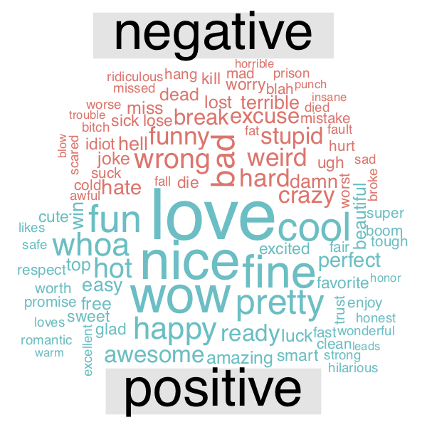
Yet another way to visualize this is a comparative word cloud.

bing_word_counts %>%
  acast(word~sentiment, value.var='n', fill = 0) %>%
  comparison.cloud(colors=c("#F8766D", "#00BFC4"), 
                   max.words=100)

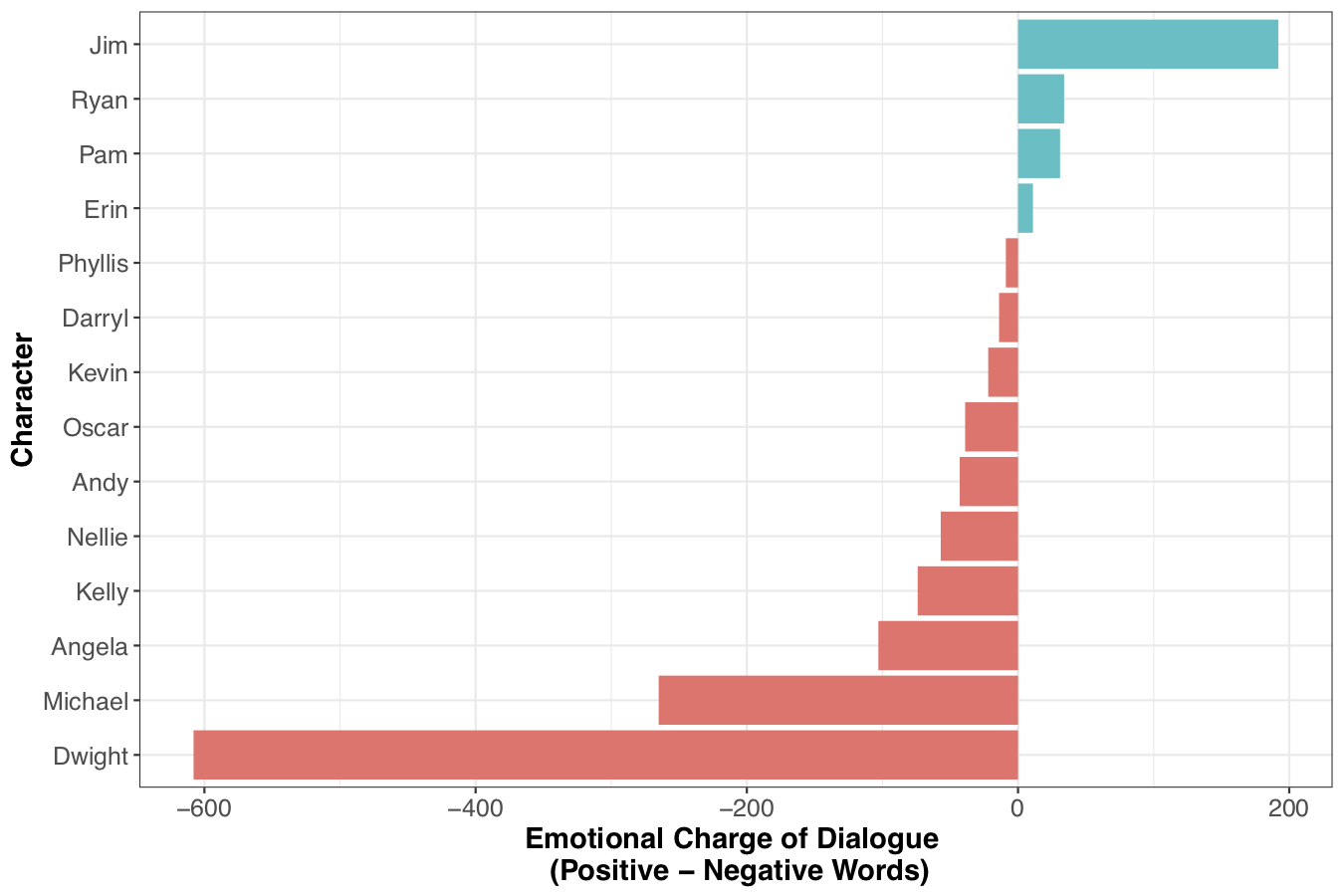
Which characters use more positive vs negative words?

First, we need to join sentiment data with the token data. I also created a variable sentimentc which subtracts the total # of negative words a character says from the total # of positive words they say.

char.sentiment= tidy.token.schrute %>%
  inner_join(sentiments, by = 'word') %>% 
  count(character, sentiment) %>%
  spread(sentiment, n, fill = 0) %>%
  mutate(sentimentc = positive-negative) 

Now, we can see which characters are are more positive vs. negative.

char.sentiment %>% 
  filter(negative +positive >300) %>%
  mutate(sent_dummy = ifelse(sentimentc<0, 'More Negative', 'More Positive')) %>%
  mutate(character = reorder(character, sentimentc)) %>%
  ggplot(aes(character, sentimentc, fill = sent_dummy)) +
  geom_col() +
  coord_flip() + 
  labs(y='Emotional Charge of Dialogue \n (Positive - Negative Words)', x = 'Character') +
  theme_bw() + 
  theme(legend.position='none', axis.text.x=element_text(size=12), axis.title.x = element_text(size=14, face = 'bold'),
        axis.text.y=element_text(size=12), axis.title.y=element_text(size=14, face='bold'))